Random Discussion (3.10)

Today we had an online seminar given by Keisuke Inomata (JHU) about the one-loop correction in scalar perturbation for SR-NSR-SR type inflation in spatially flat gauge based on his works 2502.12112 and 2502.08707. According to what he claimed, the conterterms $V_{c,(1)}$ and $V_{c,(2)}$ are defined by imposing the zero-tadpole condition $\langle\zeta\rangle=0 \quad(\zeta_n\equiv-\frac{\delta\phi}{\sqrt{2\epsilon}M_{\rm p}}, \zeta_n\simeq\zeta$ during SR period$)$.

He clearly showed that the counterterms cancel out the 1-loop contribution to the superlongwavelength perturbations sourced by $V_{(3)}$. He also claimed that he reproduced Jason&Yokoyama paper(in comoving gauge) by neglecting the contribution from tadpole and $V_{(4)}$.

During today’s Random Discussion, Xiao-Han presented a work on large non-Gaussianity in multi-brid inflation according to Atsushi & Misao’s paper 0807.0180. According to $\delta N$ formalism, the final slicing taken for the end of inflation will automatically determine the adiabatic component and the non-adiabatic component of the inflaton fields. Even if the inflation ends with an adiabatic background trajectory (only 1 degree of freedom determines everything), the choice of final slicing does matter. If we take a final slicing of inflation which is not exactly perpendicular to the background trajectory in the phase diagram, it causes the existence of the non-adiabatic component at the end of inflation.

It tells us that there is no meaning to distinguish the isocurvature and adiabatic curvature before defining the final slicing of inflation!

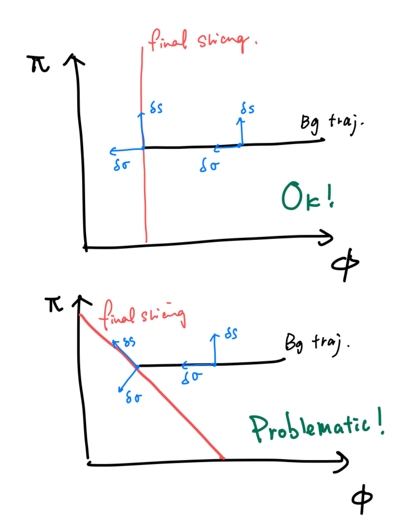
This little-known fact affects not only multi-field inflation but also single-field inflation. However, in single field inflation, we consider the end of inflation was ended in the attractor phase, i.e. $\ddot\phi$ is negligible, therefore, the condition for the end of inflation is usually given by $\epsilon_{H}=\frac{\dot\phi^2}{2}=\rm const.$. Therefore, in the phase diagram, the final slicing of inflation is perpendicular to the background trajectory in the slow roll limit $\epsilon\ll 1$. Long story short, if the inflation ends in (effective) single field slow-roll regime, the traditional way to distinguish isocurvature and adiabatic curvature works well, i.e. the component that parallels to the background trajectory is adiabatic and the component perpendicular to the background trajectory is non-adiabatic. Otherwise, the choice of end slicing does matter.

Personally, I felt that $\epsilon=1$ might not be a trivial final slicing, since at this time, the inflaton is 1) not in the attractor phase, and 2) not in the slow roll regime. Simply using $\epsilon=1$ could cause some contributions to the very short wavelength modes that exit the horizon shortly before the end of inflation.